1.原始数据
1 | #三大件 |
1 | positive = pdData[pdData['Admitted'] == 1] |
2.实现方案
- 目标:建立分类器(求解出三个参数 𝜃0𝜃1𝜃2)
设定阈值,根据阈值判断录取结果
要完成的模块
sigmoid : 映射到概率的函数
model : 返回预测结果值
cost : 根据参数计算损失
gradient : 计算每个参数的梯度方向
descent : 进行参数更新
accuracy: 计算精度
3.具体实现
3.1 sigmoid
1 | def sigmoid(z): |
3.2 预测模型-数值运算转换成矩阵运算
1 | def model(X, theta): |
3.3 数据准备
1 | # 添加一列𝜃0,指定是1 |
3.4 损失函数
将对数似然函数去负号
𝐷(ℎ𝜃(𝑥),𝑦)=−𝑦log(ℎ𝜃(𝑥))−(1−𝑦)log(1−ℎ𝜃(𝑥))
1 | def cost(X, y, theta): |
3.5 计算梯度
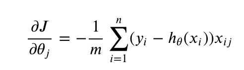
1 | def gradient(X, y, theta): |
- 3中不同梯度下降方法
1 | STOP_ITER = 0 |
1 | import numpy.random |
1 | import time |
3.6 计算精度
1 | #设定阈值 |